In 1973 Hopcroft and Karp gave a very nice  time algorithm computing a maximum matching in unweighted bipartite graphs. This algorithm turned out to be the milestone that is hard to beat. The bipartite maximum matching problem has been studied in many different flavors such as online, approximate, dynamic, randomized or the combination of the above. The HK algorithm was improved for sufficiently dense and sufficiently sparse graphs. Nevertheless, for the general case, despite of the wide interest, little improvement over HK was obtained. This is somewhat intriguing, as no reasonable example certifies that the bound for the running time of HK is in fact tight. The HK algorithm is of offline nature and relies heavily on receiving the whole graph before processing it. On the quest for making some progress on the subject matter we aimed for the dynamic setting. Say the vertices need to be matched as they show up in the graph, so some re-matching is allowed and the maximum matching needs to be maintained at all times. Can one do better than simply finding any augmenting path each time a new vertex appears?
Let us narrow down the dynamic scenario we consider: say only the vertices of one side of the graph come in online, and at the time they show up they reveal all their adjacent edges. This scenario is easily motivated as follows.
There is a set of servers and a set of jobs to be executed on these servers. Every job comes with a list of servers capable of performing the job. Of course it is reasonable to serve as many jobs as possible, hence the maximum job-server matching is highly desired. Having that motivation in mind, an online scenario seems to be the most natural: jobs come in online one at the time, and request to be matched to one of the chosen servers. We care to match the job whenever its possible, so we allow some busy servers to be reallocated.
Now the question is, what is a good way of reallocating the servers, so that the dynamic algorithm can benefit from it? We adopt the following measure: each reallocation involves some reallocating cost. We want to minimize the cost of reallocating the servers.
We associate with each server  an attribute called
  , which states how many times the server has been reallocated in the entire process. The parameter
  stands for time. We see the entire process of adding jobs as a sequence of turns, in each turn a new job appears with the list of eligible servers. The attribute describes the number of times was reallocated up to turn . These attributes guide us when we search for augmenting paths. We try to avoid servers with high ranks. This should distribute the necessary reallocations more or less evenly among the servers.
In order to follow this approach, a certain greedy strategy comes to mind. When trying to match a new job, choose the augmenting path which minimizes the maximum rank of a server along this path. This strategy has one substantial disadvantage. If any augmenting path that we can choose to match the new job contains a vertex of high rank  , then we are allowed to rematch all servers of ranks at most . That is clearly an overhead. We hence define another attribute,
  , for every job
  . This attribute says what is the rank of the lowest ranked path from to any unmatched server. When we try to match job , we search for the alternating path along which the tiers of jobs do not increase. We call such a path a tiered path. In other words, a tiered path minimizes the maximal rank on its every suffix. This seems natural: why to re-enter vertices of high rank when we can avoid them.
It turns out that this simple strategy does quite well: the ranks (and hence also the tiers) do not grow above  . That means, that each server gets reallocated at most
  times. This is already interesting. Moreover, if we knew how to efficiently choose the right augmenting paths, the total work would be
  . We have an algorithm that finds all the augmenting paths in the total time
  , what matches the offline time of HK.
So let us first take a look on how the bound on the maximum rank is obtained. First of all, we direct the edges of the graph according to the current matching: the matched edges point from servers to jobs, while the unmatched edges point the other way around. Now, directed paths are alternating, so in each turn we need to find a directed path from the new job to a free server and reverse the edges along the path. We first show that the servers of high ranks are far from the unoccupied servers: the directed distance from any server to an unmatched server in turn is at least  .
.
We now look at any set  of vertex disjoint directed paths covering all free servers in turn before applying the augmenting path. Note, that there are no outgoing edges from free servers, so the paths end there. The rank of the directed path present in the graph in turn is the maximum rank of a server on it. Let's call
  the augmenting path applied in turn
  . We analyze the augmentation process backwards. In turn , before applying , there exists a set of vertex disjoint paths
  covering free servers, such that:
- every path
 has its counterpart
  , where
  is an injection
  has rank at least as high as
  , unless 's rank is smaller or equal to one plus the rank of : then the rank of may be one less then the rank of
 - there is a path in that is not in the image of and has rank at least the rank of
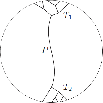
This observation may be translated as follows. Let us, for every path in , draw a vertical bar of height equal to its rank. Let us now sort the bars in descending order and put them next to each other, as shown in Figure 1 to the left. These bars are the ranks of the paths in turn . When we take a step back to turn , we have another set of bars corresponding to paths from turn , where one additional bar pops out. Moreover, some bars may have decreased by one, but all the bars that decreased are dominated (with respect to height) by the newly added bar. This is shown in Figure 1 to the right. The process ends when we reach turn  , and there is
  bars of height zero.
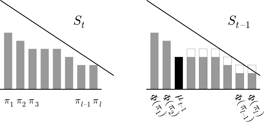
Now we move to bounding the maximum rank. The maximum rank, say  , will appear on some path in some turn
  . We take a look at set
  consisting of this single path. There is only one bar of height . In the previous turn, either there is still a bar of the height , or there are two bars of height
  . Every time the bars decrease, there comes another bar that dominates the decreased bars. Somewhere on the way back to turn there is a set of bars with the sum of heights quadratic in . The bars, however, correspond to vertex disjoint paths, and the heights of the bars are the lower bounds on the lengths of these paths. Hence, there is
  vertices in the graph and
  .
.

The question that remains is whether we are able to efficiently find these paths. The main problem here is that we need augmenting paths where the tiers of jobs along the path do not increase. This is not a good news: the tiers are difficult to maintain upon the reversal of the edges on the entire augmenting path. The idea is to maintain them in a lazy manner. For each job , instead of its actual tier, the algorithm maintains an attribute  . Subscript LB stands for lower bound, as we maintain the invariant that
 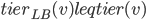 . When a new vertex turns up in some turn, is set to . The algorithm repeatedly tries to find (in the directed graph) a tiered (according to the maintained lower bounds for tiers) directed path from to a free server. It executes a search routine from , traversing only the vertices with ranks and
  's bounded by . Once a job
  with
with 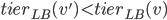 is discovered, the upper bound on the ranks and 's of vertices visited next is recursively set to
  . This goes on until one of the two things happen. It might be that a free server is discovered. Then we found an augmenting path, along which the 's of the vertices are their actual tiers (the path that we found is a witness for that). We reverse the edges along the augmenting path and increase the ranks of the reallocated servers. It might also happen that the search fails. This means, that the algorithm detects a group of vertices whose 's are lower than their actual tiers. The algorithm then rightfully increases the 's associated with these vertices. It continues the search from the point where it failed. The difference is that now it can search further, as it is allowed to visit vertices with higher 's than before. The general idea is that whenever a vertex is visited by the algorithm, either its or its rank is increased. Unfortunately upon every such visit the algorithm may touch all the edges adjacent to the visited vertex. These edges, however, will be touched in total times each. The total time amounts to .