Graph Isomorphism on graphs of bounded treewidth

Posted on November 20, 2014 by malcin

The Graph Isomorphism problem is interesting for many reasons, one being the fact that its complexity status is still unclear - it is probably not NP-complete, but not known to be in P either. In the past decades, researchers identified a large number of special graph classes for which GI is polynomial-time solvable, including planar graphs, graphs of bounded maximum degree, and graphs excluding a fixed minor, among others.

A closer look at the known algorithms for graphs of bounded degree or graphs excluding a fixed minor reveals that the dependency in the running time bound on the "forbidden pattern" is quite bad: in the first case or in the second case, for some function . Seeing such dependencies, a natural question is: do there exist fixed-parameter algorithms, parameterized by the "forbidden pattern"? In other words, does the exponent in the polynomial factor in need to depend on the pattern, on can we obtain an algorithm with running time ?

This question remains widely open for all aforementioned cases of bounded degree or excluded minor. In our recent FOCS 2014 paper, we have answered the question affirmatively for the special case of bounded treewidth graphs, proving that isomorphism of two -vertex graphs of treewidth can be tested in time .

As a starting point, observe that comparing (testing isomorphism) of two graphs together with their given tree decompositions (that is, we want to check if the whole structures consisting of a graph and its decomposition are isomorphic) can be done easily in time polynomial in the size of the graphs, and exponential in the width of the decompositions. This is a relatively standard, but tedious, exercise from the area of designing dynamic programming algorithms on tree decompositions: if you have seen a few of these, I guess you can figure out the details, but if you don't, this is probably one of the worst examples to start with, so just assume it can be done. Alternatively, you may use the recent results of Otachi and Schweitzer that say that one needs only a set of bags for the decomposition, even without the structure of the decomposition tree itself.

With this observation, the task of comparing two bounded-treewidth graphs reduces to the following: given a graph of treewidth , we would like to compute in an isomorphic-invariant way a tree decomposition of $G$ of near-optimal width. Here, isomorphic-invariant means that we do not want to make any decisions depending on the representation of the graph in the memory (like, "take arbitrary vertex"), and the output decomposition should be the same (isomorphic) for isomorphic input graphs. Given such an isomorphic-invariant treewidth approximation algorithm, we can now compute the decompositions of both input graphs, and compare given pairs (graph, its tree decomposition), as described in the previous paragraph. Note that for this approach we do not need to output exactly one tree decomposition; we can output, say, of them, and compare every pair of decompositions for two input graphs for the Graph Isomorphism problem; we only need that the set of output decompositions is isomorphic invariant.

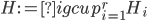
To cope with this new task, let us look at the known treewidth approximation algorithms; in particular, the arguably simplest one - the Robertson-Seymour algorithm. This algorithm provides a constant approximation in time, where is the treewidth of the input -vertex graph . It is a recursive procedure that decomposes a part of the input graph, given a requirement that a set should be contained in the top bag of the output decomposition. Think of as an interface to the rest of the graph; we will always have , but for technical reasons the set could be larger. During the course of the algorithm we maintain an invariant .

In the leaves of the recursion we have , and we output a single bag . If is small, say, , then we can add an arbitrary vertex to and recurse. The interesting things happen when grows beyond the threshold .

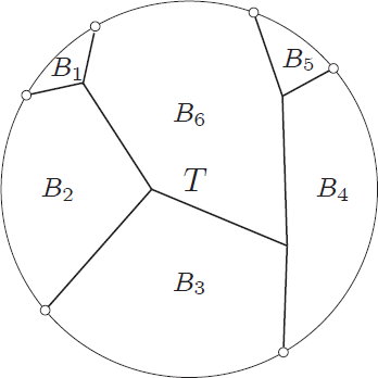
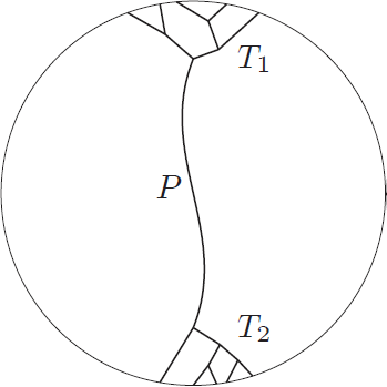
As the graph is of treewidth , but , in an optimal decomposition of the set is spread across many bags. A simple argument shows that there exists a bag , , such that every component of contains at most vertices of . The algorithm takes as a root bag (note that ), and recurses on every connected component of ; formally, for every connected component of , we recurse on with . Since every component of contains at most vertices of , in every recursive call the new set is of size at most .

In the above algorithm, there are two steps that are very deeply not isomorphic-invariant: "take an arbitrary vertex to " in the case of small , and "take any such " in the case of large . We start fixing the algorithm in the second, more interesting case.

Before we start, let us think how we can find such a set - the argument provided two paragraphs ago only asserted its existence. One of the ways to do it is to iterate through all disjoint sets of size exactly each, and check if the minimum separator between and in is of size at most (such a separator can contain vertices of or , these are deletable as well). If such a separator is found, it is a good candidate for the set - it does not necessarily have the property that every connected component of contains at most half of the vertices of , but the claim that in the recursive calls the size of the set decreased is still true. Of course, in this approach we have two not isomorphic-invariant choices: the choice of and , and the choice of the minimum separator .

Luckily, an (almost) isomorphic-invariant way to make the second choice has already been well understood: by submodularity of cuts, there exists a well-defined notion of the minimum cut closest to , and the one closest to . But how about the choice of and ?

The surprising answer is: it works just fine if we just throw into the constructed bag all separators for every choice of and . That is, we start with the tentative bag , we iterate over all such (ordered) pairs , and throw into the constructed bag the minimum cut between and that is closest to , as long as it has size at most . We recurse on all connected components of as before; the surprising fact is that the sizes of the sets in the recursive calls did not grow. To prove this fact, we analyse what happens to the components of when you add cuts one-by-one; a single step of this induction turns out to be an elementary application of submodularity. Furthermore, note that if the size of is bounded in terms of , so is the set of the bag : .

Having made isomorphic-invariant the "more interesting" case of the Robertson-Seymour approximation algorithm, let us briefly discuss the case of the small set : we need to develop an isomorphic-invariant way to grow this set. Here, we need some preprocessing: by known tricks, we can assume that (a) the input graph does not contain any clique separators, and (b) if , then the minimum cut between and is of size at most . Furthermore, observe that in our algorithm, contrary to the original Robertson-Seymour algorithm, we always maintain the invariant that and is connected. Thus, is never a clique in , and, if , we can throw into a bag the minimum cut between and that is closest to , for every ordered pair where , .

In this way, the lack of clique separators ensures that we always make a progress in the algorithm, by "eating" at least one vertex of . The bound on the size of minimum cut between two nonadjacent vertices ensures that the bag created in this way is of size , and so are the sets in the recursive calls. Consequently, our algorithm computes in an isomorphic-invariant way a tree decomposition with adhesions of size and bags of size .

Well, there is one small catch - neither of the aforementioned steps is good to start the algorithm, to provide the initial call of the recursion; the Robertson-Seymour approximation starts with just and . Here, we can start with and for every pair of nonadjacent vertices, as in this call the step with the small set will work fine. But this produces not a single isomorphic-invariant tree decomposition, but a family of decompositions - which is still fine for the isomorphism test.

A cautious reader would also notice that the described algorithm results in a double-exponential dependency on the parameter in the running time, contrary to the claim of the term. Getting down to this dependency requires a bit more technical work; we refer to the full version of our paper for details.

How pineapples help finding Steiner trees?

Posted on October 16, 2014 by sank

The Bratislava Declaration of Young Researchers is something I was involved in recently. Its preparation was inspired by Slovak Presidency of the EU and it was presented on today's informal Council of Ministers responsible for competitiveness (Research). I hope this will have some follow up, as current trend in funding research in EU is in my opinion (and not only my as this declaration shows) going in the wrong direction.
Recently with Marcin Pilipczuk, Micha? Pilipczuk and Erik Jan van Leeuwen we were able to prove that the Steiner Tree problem has a polynomial kernel on unweighted planar graphs. So far this was one of few problems where such kernel seemed possible, but existing tools (e.g. theory of bidimensionality) were unable to deliver it. Essentially, we were able to prove the following theorem.

Theorem 1. Let be a planar Steiner tree instance, and let be the cost of optimum tree connecting terminals in the unweighted graph . One can in polynomial time find a set of edges of size polynomial in that contains an optimal Steiner tree connecting in .

Figure 1. The process of cutting open the graph along the tree .

Let us shortly discuss the idea of the proof of this theorem. The most non-trivial part of it is the pineapple decomposition. In order to give you a glimpse on this decomposition we will first reduce the problem to the simpler case where all terminals lie on one designated face. Such planar graph with one designated face will be called a brick and this designated face will be called the perimeter of the brick. Without loss of generality we assume that the perimeter is the outer (infinite) face of the plane drawing of the brick. The first step of our reduction is to find 2-approxiate Steiner tree in . Next, we cut the plane open along tree (see Figure 1) to obtain the graph . Now all terminals lie on one face in whereas the optimal Steiner tree in is cut into smaller trees in each spanning some subset of terminals. As we do not know how exactly the optimal tree will be cut, we will prove that a single polynomial kernel exists for all possible subsets of terminals on the perimeter, i.e., the kernel will contain some optimal Steiner tree for every possible subset of terminals on the perimeter. This is stated in the following theorem.

Theorem 2. Let be a brick. Then one can find in polynomial time a subgraph of such that

,
is polynomial in ,
for every set , contains some optimal Steiner tree in that connects .

The idea behind the proof of Theorem 2 is to apply it recursively on subbricks (subgraphs enclosed by a simple cycle) of the given brick . The main challenge is to devise an appropriate way to decompose into subbricks, so that their ``measure' decreases. Here we use the perimeter of a brick as a potential that measures the progress of the algorithm.

Figure 2. An optimal Steiner tree and how it partitions the brick into smaller bricks .

Intuitively, we would want to do the following. Let be a tree in that connects a subset of the vertices on the perimeter of . Then splits into a number of smaller bricks , formed by the finite faces of (see Figure 2). We recurse on bricks , obtaining graphs , and return . We can prove that this decomposition yields a polynomial bound on if (i) all bricks have multiplicatively smaller perimeter than , and (ii) the sum of the perimeters of the subbricks is linear in the perimeter of .

In this approach, there are two clear issues that need to be solved. The first issue is that we need an algorithm to decide whether there is a tree for which the induced set of subbricks satisfies conditions (i) and (ii). We design a dynamic programming algorithm that either correctly decides that no such tree exists, or finds a set of subbricks of that satisfies condition (i) and (ii). In the latter case, we can recurse on each of those subbricks.

Figure 3. An optimal Steiner tree that connects a set of vertices on the perimeter of and that consists of two small trees that are connected by a long path ; note that both bricks neighbouring may have perimeter very close to .

The second issue is that there might be no trees for which the induced set of subbricks satisfies conditions (i) and (ii). In this case, optimal Steiner trees, which are a natural candidate for such partitioning trees , behave in a specific way. For example, consider the tree of Figure 3, which consists of two small trees , that lie on opposite sides of the brick and that are connected through a shortest path (of length slightly less than ). Then both faces of that neighbour may have perimeter almost equal to , thus blocking our default decomposition approach.

Figure 4. A cycle that (in particular) hides the small trees in the ring between and , and a subsequent decomposition of into smaller bricks.

To address this second issue, we propose a completely different decomposition - the pineapple decomposition. Intuitively, we find a cycle of length linear in that lies close to , such that all vertices of degree three or more of any optimal Steiner tree are hidden in the ring between and (see Figure 4). We then decompose the ring between and into a number of smaller bricks. We recursively apply Theorem 2 to these bricks, and return the result of these recursive calls together with a set of shortest paths inside between any pair of vertices on . The main technical difficulty is to prove that such circle exists. If you would like to learn more on how it works, you can still attend our talk during the coming FOCS in Philadelphia on Sunday at 11:05, or have look into the full version of the paper on arXiv. Additionally to the above result, the paper contains similar results for planar Steiner forest problem, planar edge multiway cut, as well as some generalization of these results to weighted graphs.

3 of our papers accepted for FOCS!

Posted on June 26, 2013 by sank

It seems that the 'God of FOCS' was favorable for us again and we managed to get the following 3 papers accepted for FOCS 2013:

The planar directed k-Vertex-Disjoint Paths problem is fixed-parameter
tractable, Marek Cygan, Dániel Marx, Marcin Pilipczuk and Micha? Pilipczuk, arXiv.
Improved approximation for 3-dimensional matching via bounded pathwidth local search, Marek Cygan, arXiv.
Algebraic Algorithms for b-Matching, Shortest Undirected Paths, and f-Factors, Harold N. Gabow and Piotr Sankowski, arXiv, post on the paper.

Presentation: Algorithmic Applications of Baur-Strassen’s Theorem...

Posted on October 25, 2012 by sank

The FOCS presentation for our talk on Algorithmic Applications of Baur-Strassen’s Theorem... The interesting part is the 3D interpretation of the dual LP.

Capacitated k-Centers

Posted on July 31, 2012 by cygan

During my half-year research visit at the University of Maryland, I had a chance to work with MohammadTaghi Hajiaghayi and Samir Khuller, which resulted in a paper accepted to FOCS 2012: LP Rounding for k-Centers with Non-uniform Hard Capacities (to appear in arXiv soon).

In the k-center problem, we are given an integer k and a metric dist defined on a given set of points V. The goal is to open exactly k centers, that is facilities that are to serve clients located in all the points of V, in such a way that the maximum distance between any point of V and its closest center is minimized. Simple 2-approximation algorithms are known for this problem since 80's, and by a reduction from dominating set no (2-eps)-approximation algorithm exists unless P=NP.

In the capacitated version, each point v of V is assigned its capacity L(v) and in this setting no center can serve more clients than its capacity. The special case when all the capacities are equal was studied in 90's, when Bar-Ilan, Kortsarz and Peleg gave a 10-approximation algorithm, which was later improved to 6-approximation by Khuller and Sussmann. In this paper we present a constant factor approximation algorithm for the general capacities case.

By the standard tresholding technique, one can assume that the metric dist is a shortest path metric in a given undirected unweighted graph G=(V,E). This can be achieved by guessing the value of OPT (there are only n² possibilities) and putting to the edge set all pairs at distance at most OPT. Unfortunately, even after this reduction the standard LP relaxation has unbounded integrality gap, which can be seen at the following example, where k=3 and the capacity function is uniform L(v)=4.

However, what we found surprising, when the given graph G is connected we were able to prove a constant upper bound on the integrality gap of the LP. Since one can solve the problem for each connected component of the graph independently and combine results using standard dynamic programming, a rounding algorithm for connected graphs is enough to obtain a constant factor approximation algorithm.

Let y-value of a vertex be the fraction of a center opened in it by the fractional LP solution we are working with. Since we have a sharp bound on the number of centers opened, we can not independently round y-values of vertices, because we have to preserve the sum of y-values. For this reason we use what we call chain shifting operation, where in order to move y-value between two distant vertices a and b we use intermediate fully opened (with y-value equal to one) centers as illustrated below.

Observe, that in the above figure in order to move clients between the centers we need an assumption, that all the internal vertices of the path have capacities at least L(a). This is the main obstacle in our rounding process, which clearly would not appear in the uniform capacities case. This hurdle makes our algorithm technical, as we round the fractional LP solution in several steps, where in each step we get more structure on the fractionally opened centers, at the cost of increasing distances between centers and clients those are serving.

Finally we would like to mention some open problems. The approximation ratio we obtain is in the order of hundreds (however we do not calculate it explicitly), so the natural open problem is to give an algorithm with a reasonable approximation ratio. Moreover, we have shown that the integrality gap of the standard LP formulation for connected graphs in the uniform capacities case is either 5 or 6, which we think might be an evidence, that it should be possible to narrow the gap between the known lower bound (2-eps) and upper bound 6 in the uniform capacities case.

Don't know what to do? Contract something!

Posted on July 27, 2012 by malcin

The Unique Label Cover problem (ULC for short) is the problem that the Unique Games Conjecture is about: The task is to label each vertex of a given graph with a letter from an alphabet, given constraints on edges. Each edge of the graph comes with a bijection that tells how a label on one endpoint should be translated into a label on the second endpoint. Clearly, it's trivial to verify whether all constraints may be satisfied at once; the true goal is to violate as few edges as possible. The Unique Games Conjecture treats about hardness of determining the fraction of edges that may be violated; in this post I'm going to focus on instances where we would violate only very few constraints. In other words, I'm going to study fixed-parameter algorithms for ULC parameterized by the number of violated constraints (denoted k).

The main claim of our FOCS'12 paper is that ULC problem can be solved in O(s^O(k²) n^O(1)) time for n-vertex graph and alphabet of size s. This gives that ULC is polynomial-time solvable for constant alphabet and k=O(sqrt(log(n))), improving the obvious k=O(1) algorithm. And the main technique used is very simple: If you don't know what to do, randomly contract (equivalently, make undeletable) each edge independently with probability 0.5 - maybe something interesting will be highlighted in the graph with sufficiently high probability.

What does it mean sufficiently high probability? As we are aiming at time FPT in s and k, probability of the form 1/f(s,k) is fine for us.

So, what can nice happen with such a step? First, we can observe that this is a very easy way to find good separators to recurse in Kawarabayashi-Thorup way. Without going into technical details, if we find a small (of size f(s,k)) cut that separates two large (of size at least g(s,k)) connected subgraphs, we can recurse on one of the sides. With 2^{-f(s,k)-2g(s,k)} probability we won't contract edges of the cut, while contracting a large (of size g(s,k)) connected subgraph of each side of the cut. After such operation, if two vertices of "weight" at least g(s,k) can be separated with a cut of size f(s,k), we've found a good separation.

This step needs to augment the problem with border terminals and pay attention to a few details, but the overall message is: from now on we can assume that each small (in the ULC case if suffices to say here "of size at most f(s,k)=2k") separator leaves one side of small size (in the ULC case of size roughly g(s,k)=s^k).

Let X be a solution we're looking for. We know that in G-X there is one huge connected component, and at most k (as X is of size at most k) small connected components. What do we do now? Apply the trick again! With sufficiently high probability:

each edge of X is not contracted;
each small connected component is contracted onto one vertex;
for each edge e in X and each its endpoint v that is contained in the large connected component of G-X, there are at least g(s,k) vertices contracted onto v.

The core observation now is as follows: assume the above, and let v and w be two heavy vertices: that is, on both v and w we have contracted at least g(s,k) other vertices. Since we cannot recurse, there are at least 2k+1 edge-disjoint paths between v and w; each such path gives exactly one way to translate a label of v into a label of w. With a budget of k violated constraints, we can cut only k such paths; thus, for each label of v, there is at most one reasonable label of w - the one that is yielded by a majority of paths. Thus, there are only s ways to label all heavy vertices. The rest of the algorithm is just a matter of a few small observations which we won't describe in details here.

Summing up, we found the above trick interesting, with one - not so often in the fixed-parameter tractability world - property that it is capable of handling weighted versions of the problem: it is not hard to generalize the above idea to find minimum cost set of violated constraints of size at most k. Naturally, there are a few technical devils hidden in this approach - that were sufficient to blow up the paper to 58 pages on arxiv - but still, it enabled us also to improve the k-Way Cut algorithm of Kawarabayashi and Thorup, as well as give an alternative FPT algorithm for Multiway Cut-Uncut.

We conclude with a summary of what properties are necessary to apply this approach - in case you would like to use it to you favourite problem.

First, this approach needs to be some sort of graph deletion problem, with a possibility to bypass (or make undeletable) vertices or edges
that are not to be deleted.
To make a recursive step, we need that there are only limited number of ways a solution can behave on a separator. In our algorithm we've used the fact that, in a recursive step, we need only to take care of the labeling of the separator (s^p choices for a separator of p vertices). This is closely related to the notion of finite integer index.
Finally, we need to make use of the knowledge that in the final step, the graph has very good connectivity - in the sense that a small separator can remove only a small part of the graph. In the ULC case we've observed that parts with pairwise large (of size 2k+1) flow between them have a very limited number of ways they can be labeled. This part is problem-specific, and, from our experience, is the hardest part of the algorithm.

Let's make an example of the vertex k-way cut problem, which is known to be W[1]-hard, and see what breaks in the above approach. In this problem we're given a graph and integers k and p, and we're to delete p vertices to obtain at least k connected components (we parameterize by both k and p). It is not hard to see that the recursion works perfectly well: we need to remember only how does the border vertices split into components, and how many connected components were already created. However, the last step is hard; if you look at the hardness proof, the constructed instance has already strong connectivity - you can remove only isolated vertices by small separators - but it is still capable of encoding a clique instance.

A reverse situation happens in the Bisection problem, where we're to delete k edges (k is the parameter) to obtain two halves of n/2 vertices. Here the final step seems easy, and boils down to a variant of the knapsack problem. However, in the recursive step we need to remember the balance between the parts of the graph - which gives a linear in n number of choices - and the approach breaks down. To the best of our knowledge, fixed-parameter tractability of Bisection remains open.

Algorithmic Applications of Baur-Strassen’s Theorem: Shortest Cycles, Diameter and Matchings

Posted on July 8, 2012 by sank

Finally, we were able to show how to find minimum weight perfect matchings in non-bipartite graph using matrix multiplication. This was some years of trying after my paper from ICALP 2006, where the bipartite case was solved. However, with big help of Marek Cygan and Hal Gabow we have found rather elegant solution. The algorithm is very simple and given blow. Nevertheless, the proof of it correctness is not straight forward and requires some nontrivial structural properties.

Minimum weight perfect matching algorithm:

Remove non-allowed edges from the graph, i.e., edges that do not belong to any minimum weight perfect matching,
Compute M(v) minimum weight almost perfect matching that misses the vertex v,
Define new weights of edges w’(uv) = w(uv) + w(M(u)) + w(M(v)),
Connected components of E = {uv : w’(uv)<a}, for all a, encode the family of blossoms,
Using algorithm for maximum cardinality matchings find a matching that crosses each blossom once.

This gives an algorithm working in time, where W is the maximal edge weight and ? is the matrix multiplication exponent. In the case of dense graphs with small integral weights our algorithm is faster than the O(n(m+n log n)) time algorithm of Gabow from 90 and the time algorithm of Gabow and Tarjan from 91. Previously known algorithms for this problem were using augmenting paths. This algorithm is very different and is based on structural properties that give combinatorial relation between matchings weights and the dual solution. In particular, we show that there exists a canonical dual solution that is unique.

During the work we realized that the tools developed in the paper, i.e., usage of Baur-Strassen’s theorem for the computation of allowed edges, can be used to solve other problems as well. The framework appeared to be very powerful and we were able to solve the shortest cycle problem and the diameter problem in their full generality. Previous solutions for these problems that used matrix multiplication did not handle the case of undirected graphs with negative weights. Observe that in such case even detecting whether a graph has negative length cycle is nontrivial. The Bellman-Ford algorithm does not work here as it works only in the case of directed graphs. However, the problem can be solved by a reduction to the minimum weight perfect matching problem.

After the submission we realized that some other problems can be solved using this framework. One can compute the radius of the graph, as well as solve the single source shortest path problem in undirected graph with negative weights, but without negative weight cycles. Previously known algorithm for shortest paths worked only in the case of directed graphs with negative weights.

Single Source – All Sinks Max Flows in Planar Digraphs

Posted on July 4, 2012 by lacki

This is one of the papers we got accepted to this year's FOCS. It's a joint work with Yahav Nussbaum, Piotr Sankowski and Christian Wulff-Nilsen.

The paper is about computing maximum flows in planar directed graphs. Namely, given a fixed vertex s, we show how to compute the value of the max st-flow for every vertex t. Note that we just compute the value of the flow, so the algorithm basically computes n-1 numbers. By running it n times, one can compute all-pairs max flow.

The running time is O(n log³ n). This is just a log² n factor slower than the time needed to compute a single max st-flow in a directed planar graph. In the case of undirected planar graphs, things are much easier. All-pairs max flows can be represented with a Gomory-Hu tree - in particular there can be at most n-1 distinct flow values. The representation can be found in almost linear time.

It gets more difficult in the case of planar directed graphs. Not many properties of planar flows in directed graphs are known. By switching to the planar graph dual, it's quite easy to see that the value of the max st-flow is equal to the length of the shortest directed cycle, that separates faces s* and t* and goes clockwise around t*. The latter property is the most troublesome one. While a shortest directed cycle separating s* and t* can be found easily, nobody has found a way of assuring it to be clockwise. We could just compute the shortest cycle separating s* and t*, but this way we would obtain an algorithm that finds the value of the min st- or min ts-cut, whichever one is smaller.

We use a different approach. It is based on a flow partition scheme by Johnson and Venkatesan. It basically says that if we have a separator C in the graph, such s and t lie on the different sides of this separator, then we can first compute the max sC flow (i.e. we treat all vertices of C as sinks) and the max Ct flow and then combine these two into a max st flow. It was later shown by Borradaile et al. that the procedure of combining the two flows can be implemented in time that is dependent only on |C|.

This approach is then combined with a recursive decomposition of a planar graph. Roughly speaking, a recursive decomposition is obtained by dividing the graph into two pieces using a cycle separator and then dividing the obtained pieces recursively. This gives us a tree-like structure of the separators we have used to divide the graph. Our algorithm processes this tree top-down and for each separator D, computes the max sD flow. The flow partition scheme allows us to compute the max flow to a given separator, knowing the flow to its parent in the separator tree.

A big question is now: is it also the case for the general graphs that all-pairs max flow can be found faster than by running ?(n²) max-flow computations?

4 of our papers accepted for FOCS!

Posted on July 2, 2012 by sank

We start the blog with some news that was some nice surprise for us. Lucky, we managed to get 4 papers accepted for FOCS 2012:

Algorithmic Applications of Baur-Strassen's Theorem: Shortest Cycles, Diameter and Matchings, Marek Cygan and Harold N. Gabow and Piotr Sankowski
Designing FPT algorithms for cut problems using randomized contractions, Rajesh Chitnis and Marek Cygan and Mohammad Taghi Hajiaghayi and Marcin Pilipczuk and Michał Pilipczuk
LP Rounding for k-Centers with Non-uniform Hard Capacities, Marek Cygan and Mohammad Taghi Hajiaghayi and Samir Khuller
Single Source - All Sinks Max Flows in Planar Digraphs, Jakub ??cki and Yahav Nussbaum and Piotr Sankowski and Christian Wulff-Nilsen

Some description of the papers will follow shortly.

Banach's Algorithmic Corner

University of Warsaw

Category Archives: focs